
Written by: Anish Rao, Head of Growth, Listen Labs
Key Takeaways
- Predictive brand tracking forecasts future brand health metrics from historical survey, behavioral, media, competitive, and external data.
- Models use time-aware validation on future periods instead of random splits, so accuracy reflects real decision conditions.
- The data architecture aligns survey KPIs, behavioral signals, media with adstock, competitive activity, and external controls on a shared timeline.
- Model choice depends on the goal, and dynamic regression or state-space models often beat complex ML on short tracker histories.
- Walk-forward validation and explicit lag-structure testing create forecasts with clear drivers and realistic prediction intervals.
- Listen Labs supplies wave-consistent inputs, the diagnostic “why” behind metric movement, and traceability to real respondent moments.
Definition and How Predictive Brand Tracking Works
Predictive modeling for brand tracking forecasts future brand health metrics from historical survey, behavioral, media, competitive, and external data using time-aware models validated on future periods. The goal is a defensible number with a traceable reason behind it. A correlation dressed up as a forecast fails that test.
The build follows three steps, each more specific than a generic AI overview:
- Data collection: Wave-based survey KPIs fused with behavioral signals such as search, web traffic, and purchase events, media signals such as spend, GRPs, and adstock, competitive signals such as share of voice and launches, and external signals such as macro sentiment, seasonality, and cultural moments.
- Pattern analysis: Linking those streams to perception shifts using time-aware models that respect the lag between a cause and its effect on a brand metric.
- Forecasting: Projecting awareness, consideration, and sales impact with validated prediction intervals so the brand team understands the uncertainty around each number.
This article extends an existing tracker rather than replacing it. It focuses on model selection by objective, lag-structure testing, time-based validation discipline, and operationalization into a weekly forecast dashboard.
Explore predictive brand tracking with Listen Labs
Those three steps only work if the data feeding them is aligned correctly. The next section breaks down each stream and its alignment requirement.

The Brand-Tracking-Specific Data Architecture
The data architecture for predictive brand tracking extends the existing tracker rather than replacing it. Each stream enters the model differently, and each carries a specific alignment requirement. The five streams below are ordered by how directly they feed the forecast, starting with the survey KPIs that anchor the model.
Survey KPIs are the dependent variables and the primary covariates. Wave-based awareness, consideration, favorability, NPS, and attribute batteries form the longitudinal spine of the model. Because the model treats those series as ground truth, any change to how they are measured becomes a false signal. A wording edit between waves can move a brand relevance score by more than six points, creating the appearance of a trend when the real change is minimal. That is why question consistency, audience definition, and fieldwork approach must be held constant across waves. Any change becomes a confound for the trend line and a threat to the model’s validity.
Behavioral signals such as branded search volume, web traffic, app activity, and purchase or churn events enter as covariates aligned to wave timing. Consideration tends to climb first, followed by branded search a few months later, and then business outcomes such as sales. The model needs that lag chain encoded explicitly rather than assumed away.
Media signals such as spend, impressions, GRPs, and creative flighting require adstock and saturation encoding. Brand attitude metrics rise with multiple lags of a brand’s own national traditional advertising, with the effect window extending up to five weeks of advertising lags. Without adstock, the model misattributes decaying media effects to organic brand momentum.
Competitive signals such as share of voice, competitor launch activity, and category-level sentiment enter as controls. Competitors’ ads generally reduce brand attitudes, so excluding competitor activity from the model causes it to mistake a competitor’s move for the brand’s own lift or decline.
External signals such as macro sentiment, seasonality, cultural moments, and news events require careful handling. Shifts in sentiment, usage, or consideration can be driven by pricing changes, distribution, competitor investment, or broader economic conditions, rather than by the brand itself. Including external signals as controls prevents the model from overfitting to one-off shocks.
The practical rule is simple. Every stream must be time-stamped and aligned to the wave it can actually influence. Otherwise the model leaks future information into the training set and produces forecasts that look accurate in backtesting but fail in production.
See how Listen Pulse keeps your tracker wave-consistent
Which ML Model Is Best for Predicting Brand KPIs?
There is no single best model. The right model class depends on the forecasting objective. The most common model-selection mistake in brand analytics is declaring one winner such as gradient boosting, LSTM, or ARIMA without mapping it to an objective.
The tradeoffs are real. Interpretability and accuracy often pull in opposite directions. A dynamic regression on 24 waves is explainable to a CMO. An XGBoost ensemble usually is not. Data hunger also matters on short tracker histories. Dynamic linear models are especially useful when the underlying series is latent or observed with noise, because the state-space representation separates the unobserved dynamic state from noisy measurements. That situation matches survey-tracked brand metrics measured with sampling error. A simpler dynamic regression often beats a complex model on a 24-wave tracker because it has fewer parameters to overfit and its assumptions remain transparent enough to defend.
Talk through model options with Listen Labs
Choosing a model class is only half the decision. The other half is telling the model when each cause is expected to affect the metric, which is where lag structure comes in.
Lag Structure and Leading Indicators of Brand Health
Lag structure means a cause precedes its effect on a brand metric by a measurable number of periods. Getting the lag wrong makes a good model look useless. The right variable entered at the wrong lag produces a coefficient near zero and a forecast that misses the turn.
Awareness, consideration, preference, and purchase intent typically shift six to twelve months before they show up in transaction data in most consumer categories, which makes brand metrics leading indicators of sales. Changes in brand health typically appear one to three quarters before they show up in revenue or market share. A CSAT decline typically precedes churn increases by one to two quarters.
The leading indicators of brand health differ in usefulness. Consideration and favorability tend to lead sales. Awareness moves more slowly and behaves more like a stock than a flow. If consideration has historically weakened before branded search or sales decline, a new downward trend in consideration gives marketers an opportunity to investigate before the full commercial impact appears.
Testing lag structure requires three tools applied to wave-aligned data:
- Cross-correlation functions (CCF): Identify which lags of a covariate correlate most strongly with the target metric.
- Distributed lag models: Estimate the effect of a covariate at multiple lags simultaneously, allowing the data to determine where the effect peaks.
- Granger-style lead-lag checks: Test whether past values of one series improve forecasts of another beyond what the target’s own history provides.
Lag structure determines the forecast horizon, the covariates available for use, and whether a metric behaves as a leading indicator or a lagging confirmation. A model that treats consideration as a contemporaneous predictor of sales rather than a one-to-three-quarter leading indicator will underestimate the forecast horizon and overstate real-time predictive power.
Time-Based Validation: The Rule Nobody Covers
Random splits do not work for longitudinal brand-tracking data. Random train-test splits are inappropriate for time-ordered data because they can place future observations in the training set and past observations in the test set, violating the exchangeability assumption that makes random splits valid for unrelated rows. Using standard k-fold cross-validation on time-series data routinely produces accuracy estimates that are 10–30% more optimistic than actual production performance.
The correct approach is walk-forward validation. Train on waves 1–12, predict wave 13, roll the origin forward, and repeat. Validation should simulate the exact information state that existed when a historical decision would have been made, rather than validating on a random subset of data.
Four accuracy metrics matter for brand-tracking forecasts, and each answers a different question about model performance. Report all four, because a model that looks good on one can fail on another:
- MAE (Mean Absolute Error): Average absolute error in the same units as the KPI. A MAE of 2 points on a consideration series means the model is off by 2 points on average. It treats over- and under-prediction symmetrically.
- RMSE (Root Mean Squared Error): Penalizes large errors disproportionately. A single wave off by 8 points contributes far more to RMSE than four waves each off by 2 points. The total absolute error is identical in both cases, but RMSE penalizes the single large miss.
- MAPE (Mean Absolute Percentage Error): Expresses error as a percentage of actual values. It is useful for comparing across KPIs at different scales, but penalizes underprediction more heavily than overprediction and can produce misleadingly high values for low-volume intervals.
- Directional accuracy: The proportion of waves where the model correctly predicted the direction of change. For a brand team deciding whether to act, directional accuracy often matters more than RMSE because knowing whether consideration will rise or fall next wave is more actionable than knowing the precise magnitude.
Three guardrails keep the validation honest. Hold out at least one full wave, never tune on the validation period, and re-validate every time the tracker’s question set changes. Each guardrail exists because the alternative reintroduces the data leakage that walk-forward validation is designed to prevent.
Present validation results to a skeptical stakeholder by showing the forecast error on past waves before showing the forecast. A chart of predicted versus actual consideration across the last eight waves, with MAE and directional accuracy labeled, gives the forward-looking forecast its credibility.
Prediction vs. Causation: The Boundary You Must Draw
Forecasting answers what will happen. Causal inference answers what happens if the team changes something. These questions require different methods, and conflating them creates the most expensive mistakes in predictive brand tracking.
A correlation between consideration and sales does not prove that lifting consideration will lift sales. Most business questions are causal, while most analytics outputs are associational, and conflating the two is among the most common and expensive analytical errors in industry. The practical rule is straightforward. Use predictive models to prioritize attention and causal estimates to choose actions.
When the decision involves a budget reallocation, a media plan change, or a pricing move, the right tool is marketing mix modeling or another causal method rather than a brand tracker forecast. MMM is not inherently causal unless calibrated with experiments, and traditional correlation-based MMM can miss true drivers; causal MMM anchors coefficients to experimentally validated ground truth. MMM coefficients become causal only when calibrated against periodic experimental ground truth such as lift tests or RCTs.
The causal toolkit for brand decisions includes geo-lift tests, difference-in-differences, and randomized holdout experiments. Geo-lift tests assign entire regions to treatment or control and are appropriate for channels where user-level holdouts are not practical, such as TV, out-of-home, and audio. MMM plays a different role. MMM is best suited for portfolio-level strategic questions such as allocating budget across complex mixes, quantifying long-term lagged brand media effects, and forecasting budget-shift outcomes.
Brand consideration is a stronger predictor of near-term revenue than awareness, because when a brand moves from awareness into a consumer’s active consideration set the probability of purchase increases substantially. That predictive power still does not make consideration a causal lever on its own. Acting on a correlational forecast as if it were causal, such as scaling media spend because consideration rose without a causal test, is the failure mode this boundary is designed to prevent.
Clarify prediction vs. causation with Listen Labs
Operationalization: From Model to Forecast Dashboard
A model that lives in a notebook does not help a brand team. Operationalization turns the model into something the team uses weekly, with governance that keeps the forecast defensible over time.
The forecast dashboard contains three panels that move from what will happen to why it will happen to what could change it:
- Predicted next-wave KPIs: Awareness, consideration, and favorability with prediction intervals so the team understands the uncertainty around each number.
- Predicted drivers ranked by contribution: The inputs such as media spend, share of voice, branded search, and open-ended themes that contributed most to the predicted movement, with each driver traceable to its source data.
- Scenario panel: A view of what happens to next-wave consideration if media spend increases by 20 percent, if a competitor launches, or if messaging shifts. This counterfactual layer supports planning decisions without making causal claims the model cannot support.
Connecting the model to continuous tracking means the forecast updates as new responses arrive. It no longer waits for the next wave to close. Core brand metrics such as awareness and perception can be tracked weekly or monthly, while digital signals like search, social, and traffic can be monitored daily through automated reporting. That tiered cadence keeps the model’s inputs current between survey waves.
Governance covers four questions. Who owns the model, how often it is re-fit, how forecast error is monitored, and how the dashboard handles a question-set change without breaking historical comparability. The answer to the last question matches tracker discipline. Keep core questions constant, add timely questions without altering the core instrument, and document any break in comparability as a model re-validation event.
Listen Pulse is the conversational tracker built for this operationalization problem. It runs the same study with the same screeners wave after wave, keeping the trend line clean while adding open-ended conversation and charting emerging themes alongside the KPIs teams already report. It deploys alongside an existing tracker or as the primary tracking system and integrates with Qualtrics and Decipher, so the model’s inputs stay wave-consistent and the dashboard stays connected to the research infrastructure the brand team already uses.
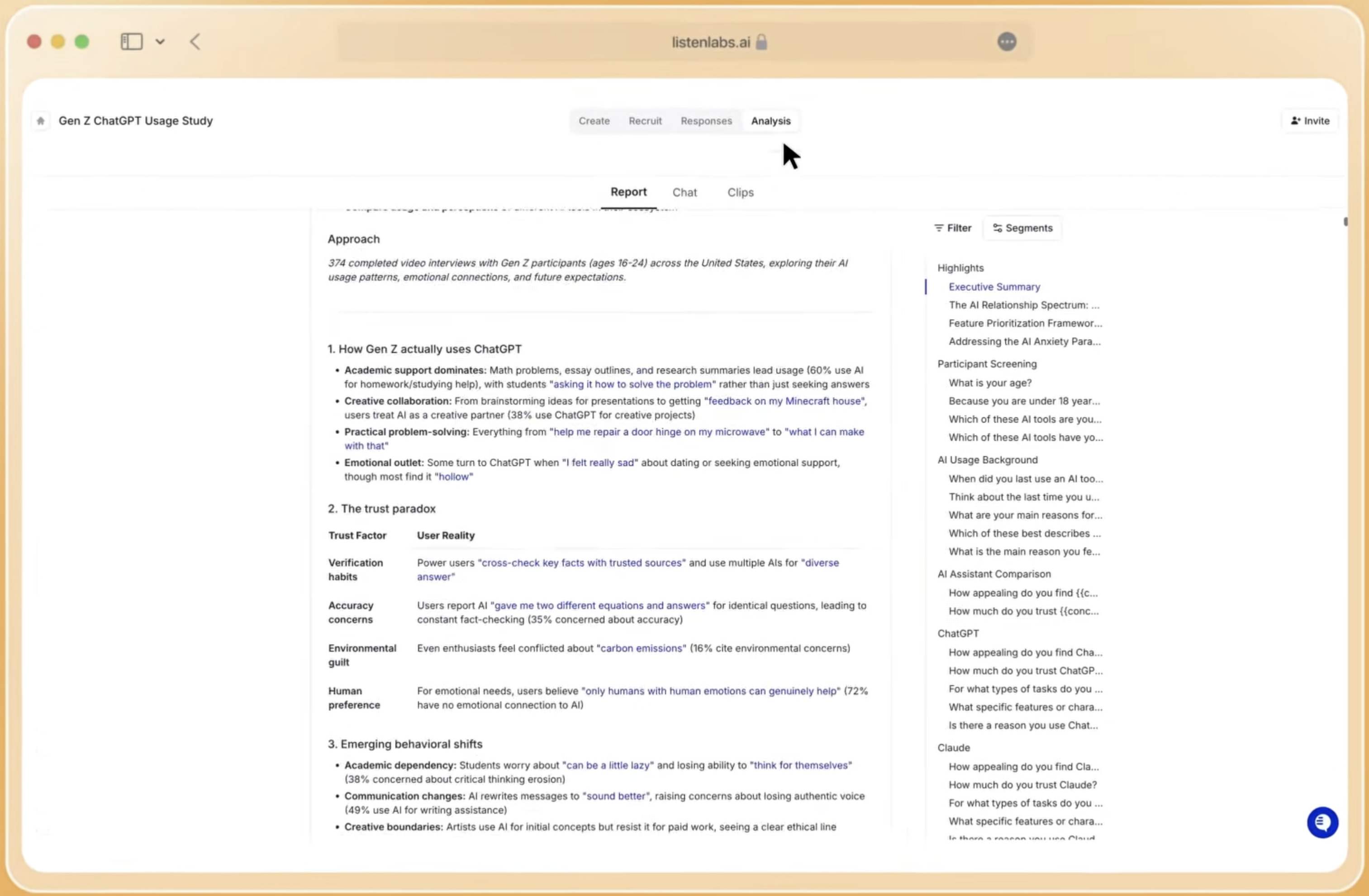
See a forecast dashboard built on Listen Pulse
Worked Example: Awareness 64%, Consideration 31%, Favorability 42%
The tracker shows awareness at 64 percent, consideration at 31 percent, and favorability at 42 percent. The model predicts a consideration decline next wave. This section walks through how the prediction was produced and why it is defensible.
Inputs that produced the prediction: Lagged consideration from the prior three waves showed a flattening trend. Branded search volume, a behavioral leading indicator, declined 11 percent over the same period. Share of voice dropped as a competitor increased media spend. Open-ended responses from the current wave surfaced a growing theme: a segment of customers describing the brand’s style as no longer matching their lives.
Lag structure that made consideration the metric to watch: Cross-correlation analysis on the historical series showed that consideration leads sales by approximately two quarters in this category, consistent with documented lag structures showing brand health changes appear one to three quarters before revenue impact. Awareness at 64 percent is moving more slowly and behaves like a stock. Favorability at 42 percent becomes the metric to watch after consideration, not before.
Validation results that justify trusting the forecast: Walk-forward validation on waves 1–20 produced a directional accuracy of 78 percent on consideration and a MAE of 1.8 points. The model correctly predicted the direction of consideration movement in 16 of 20 held-out waves. Showing that result to the CMO before the forward forecast earns the forecast credibility.
The diagnostic layer: The predicted decline traces to the open-ended theme rather than to price. This mirrors the Listen Pulse example of a well-known clothing brand famous for big logos that was quietly losing customers. Its old tracker caught the drop but could not explain it. Pulse found that style, not price, drove the shift. A growing group of customers felt the big logos were too loud for their changing lifestyles. The metric change and the reason behind it arrived in the same wave, traceable to the words, the quote, and the clip from a real person in the study.
Every number in a defensible predictive brand tracking model traces back to a real moment with a real person. That traceability separates a forecast a skeptical stakeholder will act on from one they will dismiss.
Review a worked example with Listen Labs
Predictive Brand Tracking Vs. Traditional Brand Tracking
Traditional brand trackers, the wave-based quant-only instruments from providers such as Kantar BrandZ and YouGov BrandIndex, report that a number moved but carry no diagnostic for why. Only 21% of brand leaders find their brand health insights genuinely actionable, according to Gartner’s Market Guide for Brand Health Tracking Providers. By the time a KPI declines, the underlying shift has been building for months, and explaining it requires commissioning a separate qualitative study that arrives after the response window has closed.
A typical brand tracking wave takes 8 to 12 weeks from commission to delivery, meaning the data describes a moment that has already passed by the time it is delivered. A narrative can form in a niche community, break into mainstream media, and reshape the category before the tracker reports it.
Predictive brand tracking keeps core questions constant to protect the trend line, adds open-ended conversation to every wave, and charts emerging themes next to the KPIs teams already report. The metric change and the reason behind it arrive in the same wave. The shift moves teams from reporting to forecasting plus diagnosis, and the diagnostic layer makes the forecast defensible rather than decorative.
Why Listen Labs Is The Best Solution For Predictive Modeling For Brand Tracking
Listen Labs is the best solution for predictive modeling for brand tracking because it supplies the three things that make a forecast defensible: wave-consistent inputs, the diagnostic “why” behind every metric movement, and traceability to a real moment with a real person.
Listen Pulse is the conversational tracker built for this problem. It runs the same study with the same screeners wave after wave, understands the open-ended answers, sorts them into themes, quantifies them, and charts each theme right next to the KPIs teams already report. It analyzes tens of thousands of responses 24/7. It surfaces the trends forming now, why the numbers are moving, and what is coming next. That diagnostic layer is what traditional trackers lack. Core questions stay constant to keep the trend line clean while timely questions cover new campaigns and competitors, so the model’s inputs stay comparable across waves. Every number traces back to a real moment with a real person, including their words, the quote, and the clip, which gives skeptical stakeholders the traceability they need to trust a forecast.
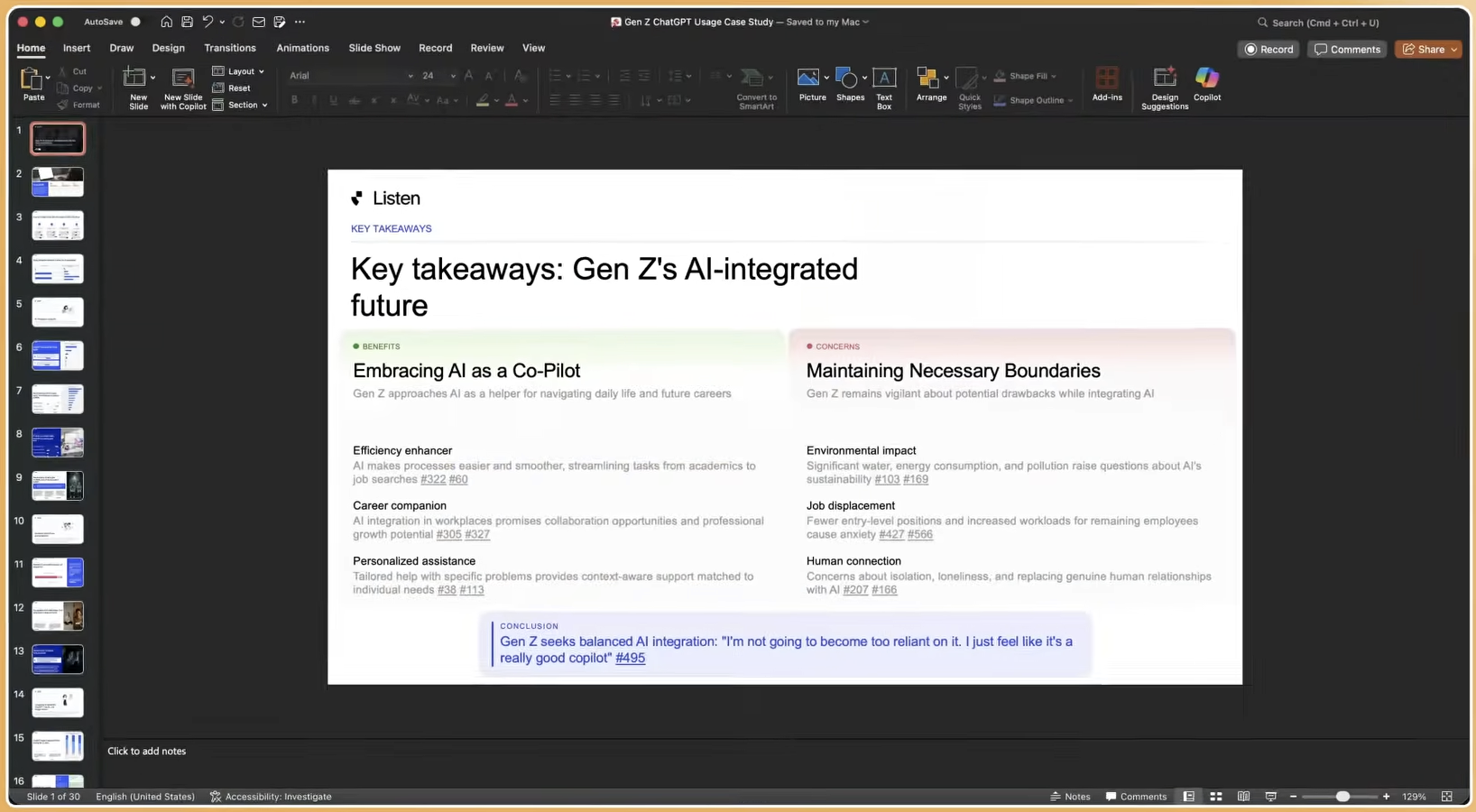
The supporting capabilities that make the forecast defensible include:
- Quality Guard: AI orchestration that matches participants on behavioral and intent data rather than only demographics, with real-time fraud detection across video, voice, content, and device signals, so the wave-consistent inputs are built on clean data.
- Emotional Intelligence: Multimodal signal analysis across tone of voice, word choice, and subconscious micro expressions, built on Ekman’s universal emotions framework, available across 50+ languages, surfacing the emotional signals that transcripts alone miss and that often precede KPI movement.
- Research Agent: One-click deliverables such as slide decks, memos, highlight reels, and charts generated from interview data in under a minute, so the diagnostic layer reaches the brand team without a six-week analysis cycle.
- Research Library: Cross-study querying in natural language, with every answer traced back to the original study, screener, and individual respondent, so the model’s inputs compound rather than expire with each project.
- Visual Insights: The AI Interviewer observes on-screen behavior and probes contradictions between stated preference and observed behavior in real time, closing the say-do gap that makes stated-preference data unreliable as a model input.
Listen Labs is the end-to-end AI research platform that sources the right participants inside its 50M+ network to conduct, analyze, and summarize thousands of in-depth customer interviews in hours, not weeks. It compresses the research cycle from 4–6 weeks to less than 24 hours, covers 45+ countries and 120+ languages, and is trusted by enterprises including Microsoft, Google, Anthropic, Sony, Sweetgreen, Perplexity, Robinhood, Procter & Gamble (P&G), Skims, Levi’s, Boston Consulting Group, and Nestlé, including roughly 15% of the Fortune 100. The platform has conducted over 1 million AI-moderated customer interviews since launch. In January 2026, Listen Labs raised a $69 million Series B led by Ribbit Capital at a valuation above $500 million, bringing total funding to $100 million after growing annualized revenue 15x to eight figures in nine months.
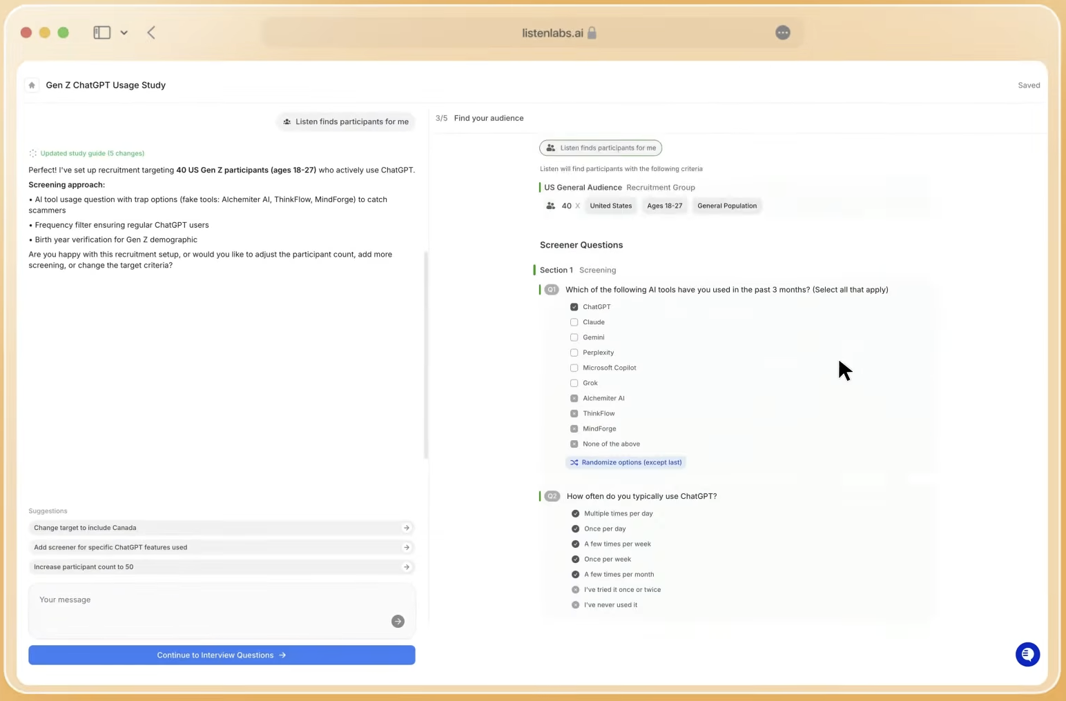
Frequently Asked Questions
What Are The Four Types Of Forecasting Models?
Time-series models such as ARIMA, exponential smoothing, and state-space extrapolate patterns in historical data forward without requiring external covariates. Causal and econometric models such as dynamic regression and marketing mix modeling incorporate external drivers like media spend, competitive activity, and macro conditions to explain and forecast metric movement. Machine learning models such as XGBoost, random forests, and neural networks identify complex nonlinear patterns in large datasets but require more data and are harder to interpret. Judgment-based and hybrid models combine statistical forecasts with expert adjustment, which helps when structural breaks or known future events fall outside the historical training window.
What Is Predictive Modeling for Brand Tracking?
Predictive modeling for brand tracking means forecasting future brand health metrics from historical and external data using time-aware models. The opening section covers the full definition and build steps. What distinguishes this approach from a standard tracker forecast is the diagnostic layer that explains why a metric is moving.
What Is an Example of a Predictive Model in Brand Tracking?
A dynamic regression model trained on 24 waves of tracker data that predicts next-wave consideration from lagged consideration, media spend with adstock encoding, share of voice, and branded search volume, validated on a held-out future wave using walk-forward validation. The model produces a point forecast and a prediction interval, with each driver’s contribution ranked so the brand team knows whether the predicted movement is driven by media, competitive activity, or an emerging theme in open-ended responses.
How Do You Validate a Predictive Brand Tracking Model?
Use walk-forward validation on time-ordered waves, as described in the validation section. The key discipline is to hold out at least one full wave and never tune on the validation period. Report the full metric set, including MAE, RMSE, MAPE, and directional accuracy, because each answers a different question about model performance.
Does Brand Consideration Actually Predict Sales?
Consideration tends to move ahead of sales, though the lead time varies by category and should be established from your own tracker’s history rather than assumed. The causation section explains why a correlational forecast cannot answer a counterfactual question. The practical takeaway is to use causal methods such as marketing mix modeling calibrated with geo-lift tests, randomized holdout experiments, or difference-in-differences when the decision requires a counterfactual about sales.
How Is Predictive Brand Tracking Different from a Traditional Brand Tracker?
Traditional trackers are wave-based and quant-only, so they report that a number moved but carry no diagnostic for why. By the time a KPI declines, the underlying shift has been building for months, and explaining it often requires a separate qualitative study. Predictive brand tracking keeps core questions constant to protect the trend line, adds open-ended conversation to every wave, and charts emerging themes next to the KPIs teams already report. The metric change and the reason behind it arrive in the same wave, shifting teams from reporting to forecasting plus diagnosis.
Can You Forecast Brand Health Without a Long Historical Dataset?
Yes, but with caveats. State-space models with weakly informative priors on variance components can stabilize inference on short series because the prior provides structure the data cannot yet supply. Simpler dynamic regression models often outperform complex models on short tracker histories because they have fewer parameters to overfit. The minimum viable history depends on the forecast horizon, the number of covariates, and whether the series contains a full seasonal cycle. A tracker with fewer than eight waves should use simpler model classes and wider prediction intervals and should be explicit with stakeholders about the uncertainty that short history introduces.
How Do You Handle A Question-Set Change Without Breaking The Trend Line?
Keep core questions constant across waves to protect the trend line. Add timely questions for new campaigns and competitors without altering the core instrument, and document any break in comparability as a model re-validation event.